Introduced in OTP 21, the :scheduler module adds some really convenient ways to figure out how hard the BEAM is working.

Essentially, it allows you to take samples of the scheduler_wall_time and use those to figure out scheduler utilization over a period of time.

Why is “scheduler utilization” important? Well, in order to provide maximum responsiveness, the BEAM does busy-waiting while not under heavy load, which can make the OS think the BEAM is hard at work, when it really isn’t. If you’re getting metrics based solely on OS cpu usage, you might not have the most accurate picture of the state of your system. This is where scheduler utilization comes in.

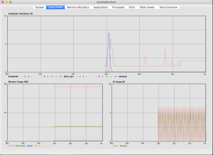
If that term sounds familiar, if might be because it’s one of the three graphs on :observer’s Load Charts pane.

Scheduler utilization is calculated from the scheduler_wall_time statistic, which looks at how much “actual” work the schedulers are doing.

To learn more, you can checkout §5.1.2 of Fred Hebert’s fantastic (and amazingly free) e-book Erlang in Anger.

scheduler_wall_time is really important but isn’t super useful data at a glance.

iex(1)> :erlang.statistics(:scheduler_wall_time)
[
  {2, 8336418000, 2047725653000},
  {4, 33739000, 2047725633000},
  {3, 87774000, 2047725632000},
  {1, 8290619000, 2047725614000},
  {5, 48000, 2057243093000},
  {6, 8000, 2057243093000},
  {7, 15000, 2057243093000},
  {8, 670000, 2057243094000}
]

So, up until OPT 21, we would have to manually convert that data into more readable scheduler utilization data, usually using an algorithm described in the Erlang docs.

But thanks to OPT 21 and the :scheduler module, no more!

iex(2)> :scheduler.sample() |> :scheduler.utilization()
[
  {:total, 0.140625, '14.1%'},
  {:normal, 1, 0.7413793103448276, '74.1%'},
  {:normal, 2, 0.15789473684210525, '15.8%'},
  {:normal, 3, 0.09523809523809523, '9.5%'},
  {:normal, 4, 0.11764705882352941, '11.8%'},
  {:cpu, 5, 0.0, '0.0%'},
  {:cpu, 6, 0.0, '0.0%'},
  {:cpu, 7, 0.0, '0.0%'},
  {:cpu, 8, 0.0, '0.0%'}
]

And even better. We can take two samples, an arbitrary amount of time apart, and calculate the scheduler utilization for that window of time. In the example below, I’ll take a sample, run some CPU intensive code, wait for it to finish, take another sample, and then calculate the scheduler utilization for the time in between.

iex(3)> doing_work = fn() -> Enum.reduce(1..10_000_000, 1, fn(x, acc) -> x + acc end) end
#Function<21.91303403/0 in :erl_eval.expr/5>
iex(4)> sample_1 = :scheduler.sample()
{:scheduler_wall_time,
 [
   {:normal, 1, 25000, 36000},
   {:normal, 2, 7000, 37000},
   {:normal, 3, 7000, 31000},
   {:normal, 4, 6000, 29000},
   {:cpu, 5, 48000, 9517515000},
   {:cpu, 6, 8000, 9517516000},
   {:cpu, 7, 15000, 9517517000},
   {:cpu, 8, 670000, 9517517000}
 ]}
iex(5)> tasks = Enum.map(1..2, fn(_) -> Task.async(doing_work) end)
[
  %Task{
    owner: #PID<0.417.0>,
    pid: #PID<0.421.0>,
    ref: #Reference<0.2323078148.1871183874.104832>
  },
  %Task{
    owner: #PID<0.417.0>,
    pid: #PID<0.422.0>,
    ref: #Reference<0.2323078148.1871183874.104833>
  }
]
iex(6)> Enum.map(tasks, fn(x) -> Task.await(x) end)
[50000005000001, 50000005000001]
iex(7)> sample_2 = :scheduler.sample()
{:scheduler_wall_time,
 [
   {:normal, 1, 7841326000, 15958502000},
   {:normal, 2, 7815658000, 15958421000},
   {:normal, 3, 85503000, 15958536000},
   {:normal, 4, 31551000, 15958553000},
   {:cpu, 5, 48000, 25475894000},
   {:cpu, 6, 8000, 25475894000},
   {:cpu, 7, 15000, 25475894000},
   {:cpu, 8, 670000, 25475895000}
 ]}
iex(8)> :scheduler.utilization(sample_1, sample_2)
[
  {:total, 0.12355537993253109, '12.4%'},
  {:normal, 1, 0.4913568133679014, '49.1%'},
  {:normal, 2, 0.48975203253662775, '49.0%'},
  {:normal, 3, 0.005357394066674792, '0.5%'},
  {:normal, 4, 0.001976686565750066, '0.2%'},
  {:cpu, 5, 0.0, '0.0%'},
  {:cpu, 6, 0.0, '0.0%'},
  {:cpu, 7, 0.0, '0.0%'},
  {:cpu, 8, 0.0, '0.0%'}
]
iex(9)> :scheduler.utilization(sample_1)
[
  {:total, 0.04114374972569954, '4.1%'},
  {:normal, 1, 0.1632406090988541, '16.3%'},
  {:normal, 2, 0.16345000400638107, '16.3%'},
  {:normal, 3, 0.0017907787879334676, '0.2%'},
  {:normal, 4, 6.684305418624684e-4, '0.1%'},
  {:cpu, 5, 0.0, '0.0%'},
  {:cpu, 6, 0.0, '0.0%'},
  {:cpu, 7, 0.0, '0.0%'},
  {:cpu, 8, 0.0, '0.0%'}
]
iex(20)> :scheduler.utilization(sample_2)
[
  {:total, 1.5842515324913467e-4, '0.0%'},
  {:normal, 1, 6.205913888450464e-5, '0.0%'},
  {:normal, 2, 0.0011720571108540937, '0.1%'},
  {:normal, 3, 1.62829995663036e-5, '0.0%'},
  {:normal, 4, 1.700096098506325e-5, '0.0%'},
  {:cpu, 5, 0.0, '0.0%'},
  {:cpu, 6, 0.0, '0.0%'},
  {:cpu, 7, 0.0, '0.0%'},
  {:cpu, 8, 0.0, '0.0%'}
]

Isn’t that cool?! Even though the load isn’t represented at all in the samples themselves, in the result of :scheduler.utilization(sample_1, sample_2) it definitely is. Awesome!